
Note on the sensor: For this post, we used a Gen 1 OS1-64 running firmware 1.12. Please check out our YouTube channel to have a look at the latest data output of our updated sensors.
The purpose of this project was to develop a Machine Learning model to enable an RC car to autonomously navigate a race track using an Ouster OS1 lidar sensor as the primary sensor input. The model is an end-to-end Convolutional Neural Network (CNN) that processes intensity image data from the lidar and outputs a steering command for the RC car.
This is inspired by the Udacity Self Driving Car “behavior cloning” module as well as the DIY Robocars races. This project builds upon earlier work developing a similar model using color camera images from a webcam to autonomously navigate the RC car.
This post covers the development of a data pipeline for collecting and processing training data, the compilation and training of the ML model using Google Colab, and the integration and deployment of the model on the RC car using ROS.
Platform Overview
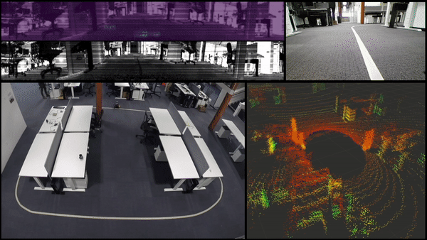
For this project, the base RC platform is the Exceed Blaze (Hyper Blue) vehicle. To mount the hardware, the platform was modified with the Standard Donkey Car Kit. The complete system is shown in the image below.
For sensing, we will be using an Ouster OS1-64 lidar sensor. The system also has a Genius WideCam F100 webcam and an OpenMV Cam M7 mounted but they were not used for this project.
Lidar sensors traditionally output a 3D pointcloud which contains rich spatial information. However, this data is more challenging to work with compared to camera images in ML applications. The blog post, “The Lidar IS the Camera” details how the OS1 lidar is able to output fixed resolution depth images, signal images, and ambient images in real-time, all without a camera. The open source driver outputs these data layers as fixed resolution 360° panoramic frames. This results in camera-like images that can be used with the same ML models developed using a color camera. As the blog post states,
“The OS1 captures both the signal and ambient data in the near infrared, so the data closely resembles visible light images of the same scenes, which gives the data a natural look and a high chance that algorithms developed for cameras translate well to the data.”
All processing is done on a Compulab fitlet2 with an Arduino Uno providing commands to the motors for steering and throttle via a PCA 9685 Servo Driver. The vehicle can be operated remotely with an Xbox controller.
The Compulab fitlet2 runs Ubuntu 18.04 as the base operating system. ROS is used as the middleware, providing inter-process communication between the software components as well as robot-specific libraries and visualizers. For the ML model development, Tensorflow and Keras are used with Google Colab providing the training environment.
Previous Work
One of the primary motivations of this work was to determine if the camera-like images from the OS1 lidar sensor could be used in a ML model architecture originally intended on color camera images.
Previously, the same hardware and software system was used to develop and verify a ML model using color camera images to reliably navigate the RC car around a similar racetrack.
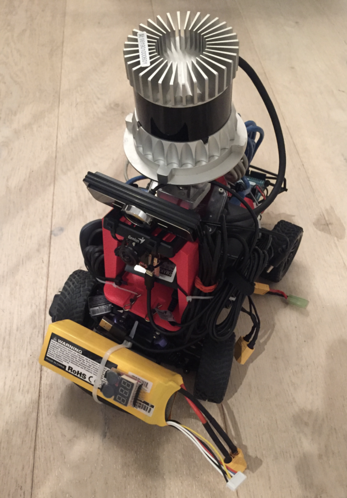
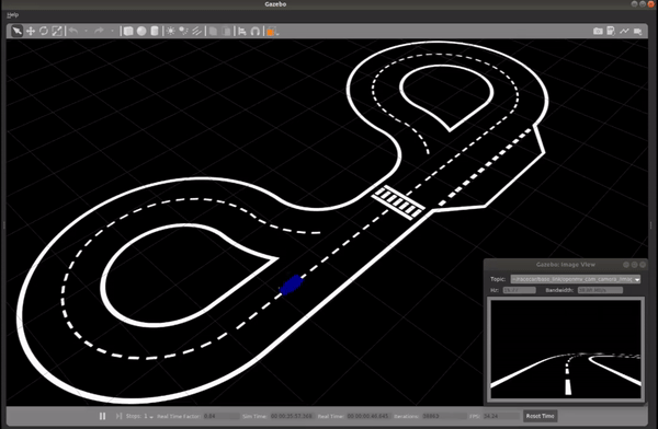
Before using the real-world hardware, a simulated environment was used to validate the data pipeline, model training, and model deployment process. ROS Gazebo was used as the simulation environment and RViz was used to visualize the simulated camera output.
To generate simulated images, a simulated RGB color camera was mounted on a simulated RC car provided by the MIT RACECAR project.
A simulated Ouster OS1 was also mounted on the vehicle but not used at the time. The post, “Simulating an Ouster OS-1 lidar Sensor in ROS Gazebo and RViz” details the process of simulating an Ouster OS1 sensor using ROS.
Lastly, the Conde world file developed by Valter Costa for his paper, “Autonomous Driving Simulator for Educational Purposes” was used as the simulated environment to operate the system and serve as a test track for training.
To collect training data, the simulated vehicle was manually driven around the track and the steering commands and simulated images were recorded in ROS bag format.
The data was then processed and used to train the ML model. For this application, the model developed by Nvidia and described in their blog post, “End-to-End Deep Learning for Self-Driving Cars” was implemented. They develop a convolutional neural network (CNN) to map raw pixels from a single front-facing camera directly to steering commands.
A ROS node was developed to use the trained ML model for inference. In the simulation environment, the ML model processed simulated color camera images and output steering commands to control the vehicle verifying the data pipeline, model training, and model deployment process.
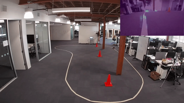
The process was repeated in the real world, collecting training data around a track, training the model, and deploying the model on the physical platform. The system performed successfully, navigating the RC vehicle around the track autonomously as shown below.
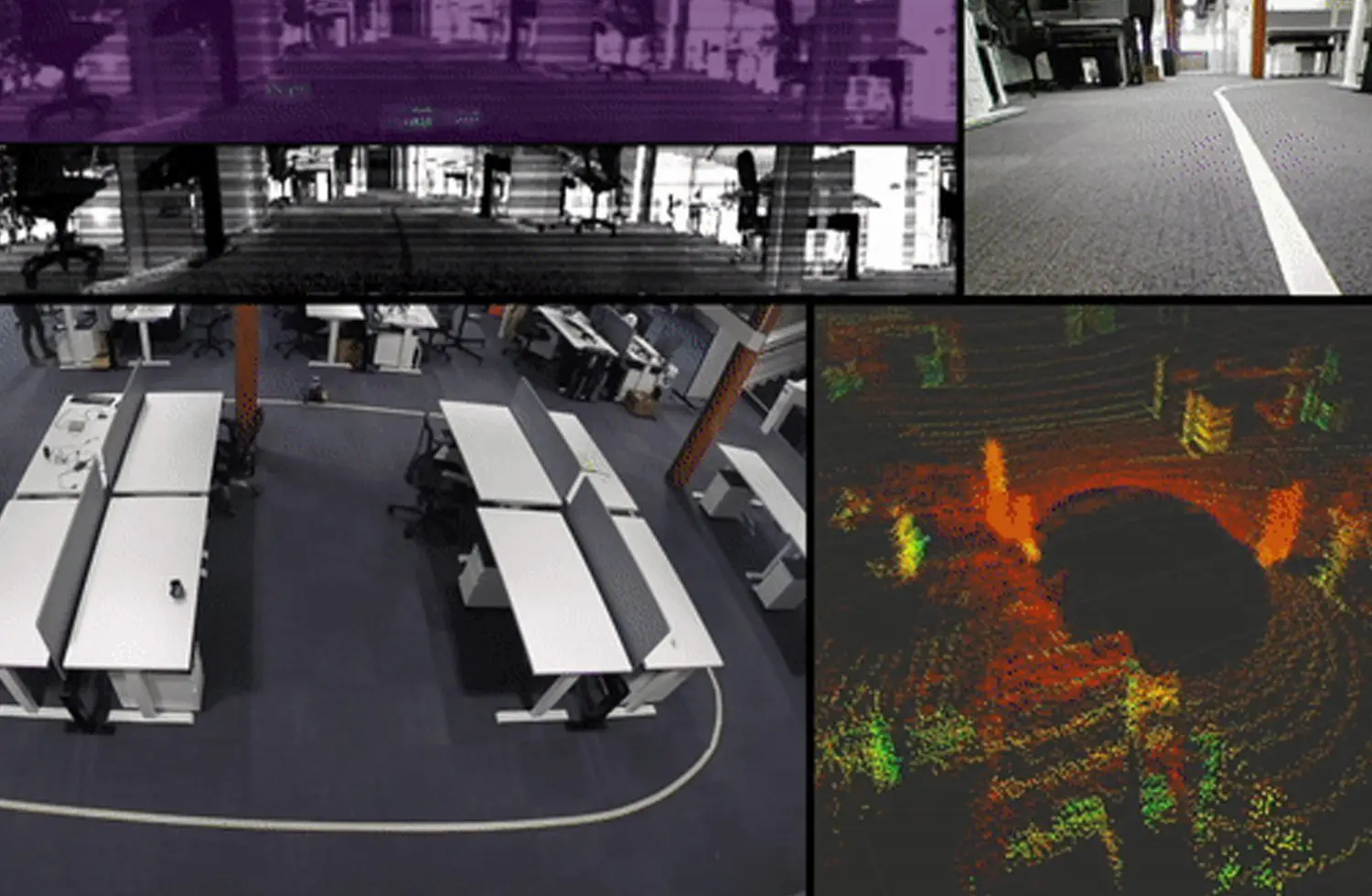
Real World Data Collection
Once the system was verified using color camera images, the next step was to adapt the system for the Ouster OS1 data. When working with the RC car, the diy_driverless_car_ROS repository is used, specifically the rover_ml package.
When manually operating the RC car, the rc_dbw_cam.launch launch file is used to start the system. For this project, the OS1 was operated in 1024×20 mode. The higher frame rate was used to more closely match the color camera’s framerate.
$ roslaunch rover_teleop rc_dbw_cam.launch os1:=true ekf:=false
The record_training.sh script is used to record the training data.
$ source record_training.sh
The primary topics of interest are the steering commands published on the /racecar/ackermann_cmd_mux/output topic and the lidar intensity channel image on the /img_node/intensity_image topic.
The vehicle was manually maneuvered around the track for a total of 10 laps, 5 in each direction.
Once we’ve collected the training data, it needs to be organized and processed. This involves extracting the lidar image data and steering command data from the ROS bag and saving it in a format that is easier to manipulate with Tensorflow and Keras.
The lidar images are saved as JPG files with unique filenames based on the timestamp they were recorded. The steering commands are also extracted and stored in a CSV file. Each row in the CSV file lists the image filename as well as the steering and throttle values associated with that image. Since the lidar images and steering commands are published at different frequencies, a basic interpolation is performed to estimate the steering command at the time each lidar image was captured.
To execute the transformation, the rosbag_to_csv.py script is used. This is a slightly modified version of Ross Wightmans bagdump.py script.
This CSV file (interpolated.csv) and the associated JPG images form the basis of our training data set. An example of the CSV output is shown below.
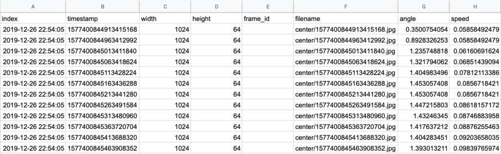
The result is a local directory of lidar images and an interpolated.csv file correlating image file names with the associated steering angle command. The data is then archived in a .tar file for use with Google Colab.
Data Processing and Model Training in Google Colab
This section describes the process of using Google Colab for the model training process instead of the embedded device on the RC car. Depending on the size of the dataset or the complexity of the model, it can be difficult to train a ML model on an embedded device.
Google Colab is a free research tool for machine learning education and research. It’s a Jupyter notebook environment that can be accessed via a web browser. Code is executed in a virtual machine that has 12GB of RAM and 320GB of disk space. Google Colab offers free use of GPUs and now provides TPUs as well. This makes them a great tool for training ML models with large data sets.
Google Colab Notebook Setup
We will use the Development of an End-to-End ML Model for Navigating an RC car with a Lidar notebook to process the dataset, train the ML model, and evaluate the ML model’s performance. First, we want to make sure the runtime environment is properly setup. From the Runtime menu, select the option to Change runtime type to get to the Notebook settings menu.
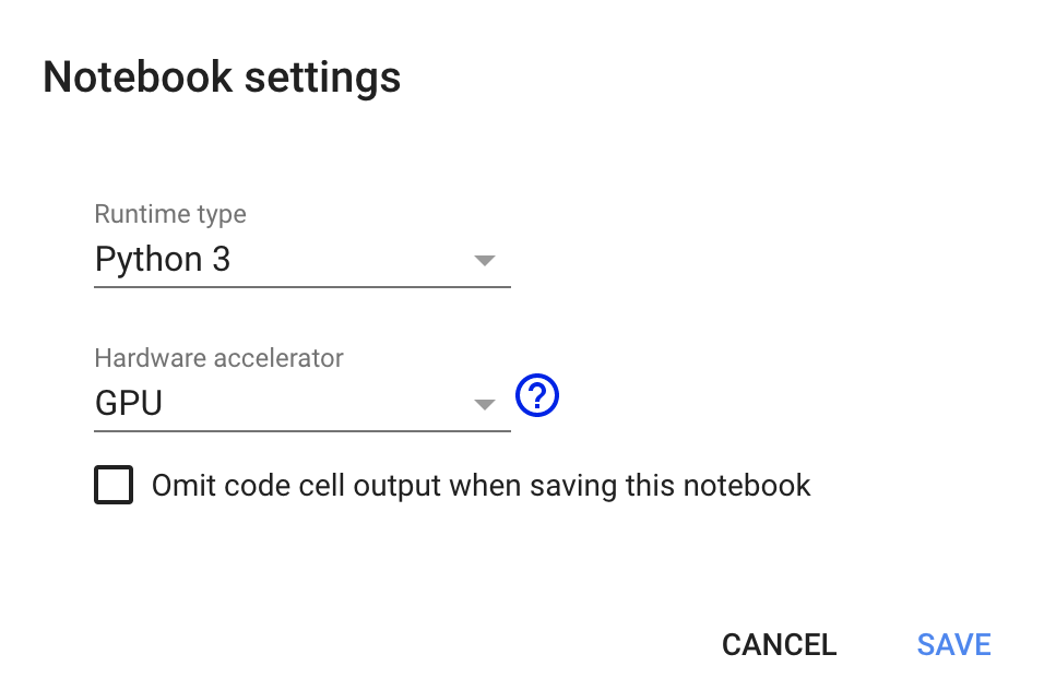
The notebook is compatible with Python 2 or Python 3 but make sure GPU is selected in the Hardware Accelerator dropdown.
Once the notebook is properly setup, we can begin executing the notebook. The notebook is not compatible with TF2.0 at this time. The command %tensorflow_version 1.x ensures that TF1.0 is used instead of TF2.0. The cell outputs the Tensorflow and Keras versions loaded.
Tensorflow Version: 1.15.0Tensorflow Keras Version: 2.2.4-tf
Finally, we confirm that the GPU we selected is available. If the GPU is available, the name is also printed. Currently, a Nvidia Tesla P100 is available.
Dataset Processing
Once the notebook is properly configured and the environment setup, we can start loading the dataset to be used for training.
The dataset is stored as a .tar file hosted on AWS. The dataset is downloaded and extracted into the Colab environment.
Next, we parse the interpolated.csv file and load the information into a Pandas dataframe. A summary of the dataframe is provided as the cell output.
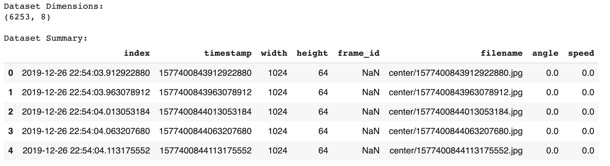
This dataset has over 6,000 samples.
Next, we want to process the dataset itself. This involves removing unused columns, any NULL values, and any entries with a 0 throttle value. We only want the model to be trained on data where the RC car was moving.
We can visualize the distribution of the steering commands using a histogram. The widget allows the user to select the number of bins to use for the histogram. Using the default of 25 bins produces the histogram below.
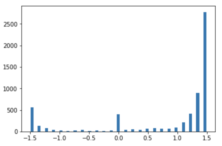
It’s evident that the data set contains an uneven distribution of steering commands.
We can normalize this distribution to have a more uniform distribution to ensure that the ML model is trained on a variety of inputs and doesn’t overfit. If the hist checkbox is selected, the dataset is pruned so that no more than a certain number of entries exist per bin. This value is set using the samples_per_bin variable and is default to 150. The histogram of the remaining entries is plotted, which looks much more uniform than the original histogram.
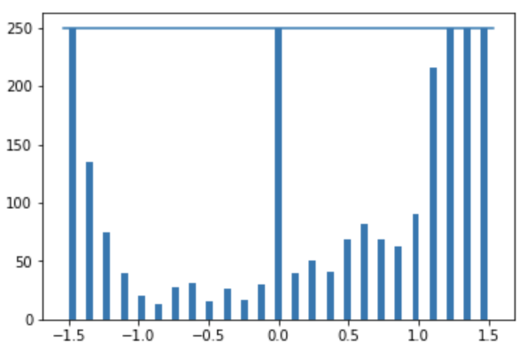
Image Processing
Once the dataset is normalized, we can move on to evaluating the quality of the images by visualizing them. There are several steps we will take to process the images.
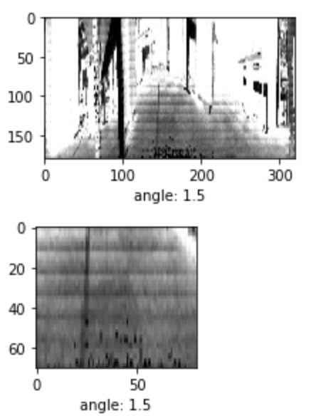
First, we will resize the images from their native 1024×64 to 320×180. While this does alter the native aspect ratio, the details that may be lost in the images aren’t valuable for this task. The image is also cropped to remove regions of the image that aren’t relevant to the training task. This prevents the model from learning features that are unique to the environment.
The image below shows the original image, resized to 320×180, as well as the cropped version. The cropped image retains the floor and lane while removing the rest of the office environment.
These image processing functions will be incorporated into subsequent steps in the ML model definition and training process.
Define Training and Validation Datasets
Once the dataset is processed and reviewed, we need to split that data into a training set and a validation set. The training set is the data that is used to adjust the weights of the model during training. The validation set doesn’t impact the model weights, but is used to verify that the model isn’t overfitting on the training data.
Before splitting the dataset, we will explore data augmentation. Since our dataset is relatively small, we can use data augmentation techniques to generate slightly modified versions of our dataset for training and vastly expand the dataset. This can make the final model more accurate and more robust to changes in the environment.
Keras provides the ImageDataGenerator class which has several built-in functions for manipulating images. This includes shifting the image vertically or horizontally, zooming in on the image, or adjusting the brightness. The post, “Exploring Image Data Augmentation with Keras and Tensorflow” provides a good overview of the options with examples of each.
When working with large datasets, it’s helpful to use Keras data generators to handle loading the data. These are specifically helpful when manipulating datasets containing images. For this example, we will define our own basic data generator. In the future, we can use the Keras implementations such as the ImageDataGenerator class.
The data generator will take in a dataset of sample data as well as the batch size hyperparameter value and a flag to determine if the data should be augmented.
def generator(samples, batch_size=32, aug=0)
The data generator loads an image and resizes it. It then loads the steering angle command associated with that image. If the aug flag is enabled, it performs basic image augmentation using the augmentation data generator. With or without augmentation, the image and the angle are then stored in separate arrays. These are shuffled and then returned.
yield sklearn.utils.shuffle(X_train, y_train)
Finally, we use the train_test_split function from the sklearn library to split our dataset into training and validation samples.
train_samples, validation_samples = train_test_split(samples, test_size=0.2)
We use 80% of the data for training and 20% validation. This ends up being around 2,900 training samples and 700 validation samples.
These are input into our dataset generator function resulting in a training data generator and a validation data generator.
train_generator = generator(train_samples, batch_size=batch_size_value, aug=1)validation_generator = generator(validation_samples, batch_size=batch_size_value, aug=0)
Model Architecture and Training
As described previously, a model developed by Nvidia is used to map raw pixels from the lidar image directly to steering commands.
The network consists of 9 layers, including a normalization layer, 5 convolutional layers, and 3 fully connected layers. A visualization of the model from the paper is shown below:
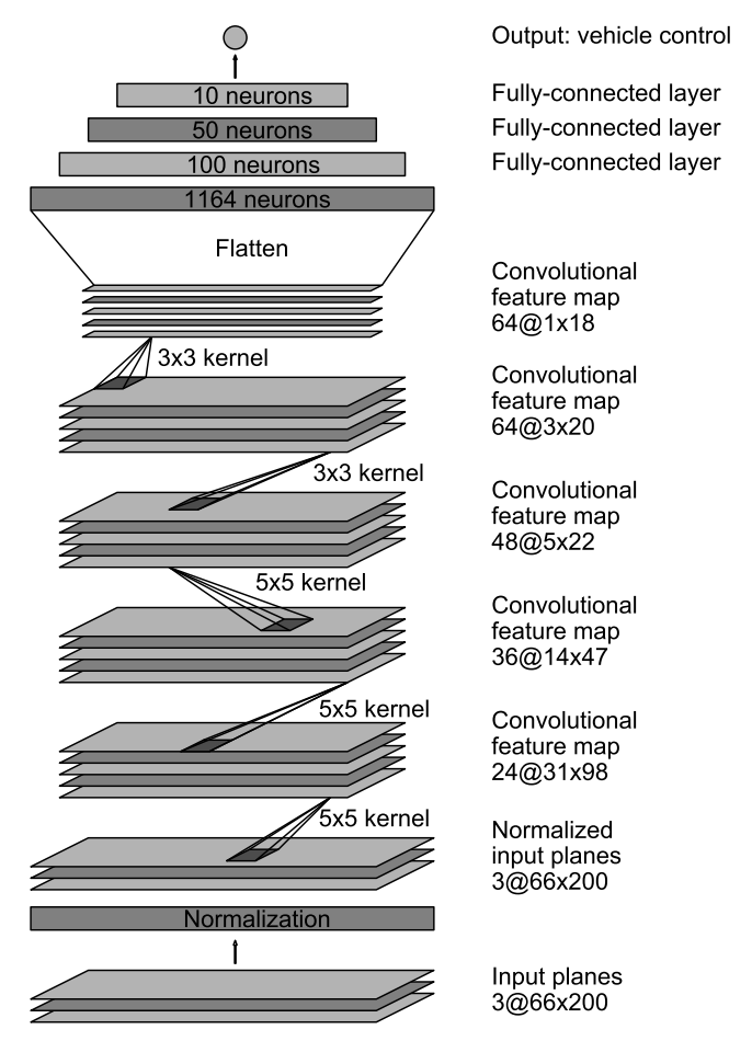
This model is compiled using the Keras API. The input image is trimmed using the cropping values discovered previously.
model.add(Cropping2D(cropping=((height_min,bottom_crop), (width_min,right_crop)), input_shape=(180,320,3)))
The next function performs some basic preprocessing of the incoming data. The image is normalized so the pixel values are centered around zero with a small standard deviation.
model.add(Lambda(lambda x: (x / 255.0) - 0.5))
The remaining lines define the specific model layers. Once the model is defined, the model is compiled.
model.compile(loss='mse', optimizer=Adam(lr=0.001), metrics=['mse','mae','mape','cosine'])
The Mean Squared Error is specified for the loss function to minimize during training. This metric is useful for regression tasks. The Adam optimizer is specified for the optimizer argument.
This results in a model with 701,559 trainable parameters.
Before training, several callbacks are also defined. Callbacks are utility functions that are triggered and called during the model training process.
First, checkpoints are setup. This stores the model weights during the training process so the model can be re-loaded if the system. This is useful in the Colab environment because the instances can disconnect after a certain timeout period.
checkpoint = ModelCheckpoint(filepath, monitor='val_loss', verbose=1, save_best_only=True, mode='auto', period=1)
The EarlyStopping callback is used to end the training process if the model performance plateaus. This helps prevent overfitting. The ReduceLROnPlateau function is similar. If the model performance stops improving, the learning rate of the Adam optimizer is automatically adjusted.
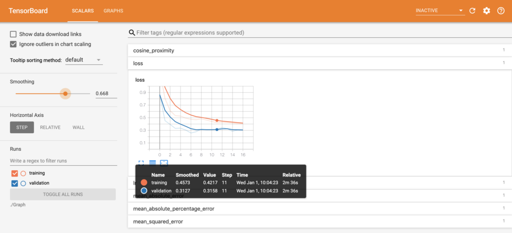
Lastly, Tensorboard is configured. TensorBoard is a visualization tool provided with TensorFlow. It enables tracking experiment metrics like loss and accuracy as well as visualizing the model graph. When executing the cell, a link is provided in the output to the Tensorboard instance. An example image of Tensorboard during the training process is shown below.
Once the model is compiled and the set of callbacks defined, the model is ready for training. Before training, several hyperparameters are defined.
First, the step sizes for the training and validation data are defined.
steps_per_epoch=(len(train_samples) / batch_size_value)validation_steps=(len(validation_samples) / batch_size_value)
This defines the total number of steps (batches of samples) to yield from the data generator before declaring one epoch finished and starting the next epoch.
Next, the number of epochs is defined.
n_epoch = 50
Finally, the fit_generator function is used to start the model training process.
history_object = model.fit_generator(generator=train_generator,steps_per_epoch=STEP_SIZE_TRAIN,validation_data=validation_generator,validation_steps=STEP_SIZE_VALID,callbacks=callbacks_list,use_multiprocessing=True,epochs=n_epoch)
Once training begins, the cell will output the metrics for each epoch. Once training is complete, the model can be saved to the Colab instance for download to a local workstation.
Model Evaluation
The model training process provides some insight into the model’s performance via the performance metrics that are output. However, to better understand how the model will perform, the trained model can be used to make predictions on some of the sample data and view the results.
The training performance can be visualized by plotting the loss function for both the training and validation datasets during the training process.
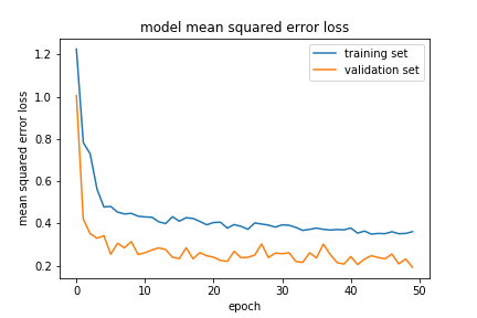
It’s evident that the loss drops quickly in the beginning but the improvement slows as the training process continues. Both the training and validation plots are similar, indicating the model is not overfitting on the data.
Next, the model can be used to predict steering command values for each of the images in the subset of data. The predicted values will be compared to the known true values and the error will be visualized.
First, the error can be visualized as a histogram.
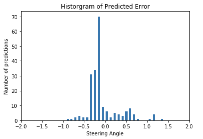
The error seems to be pretty evenly distributed with the majority of the errors near 0 which is good.
Also, the error can be visualized as a scatter plot.
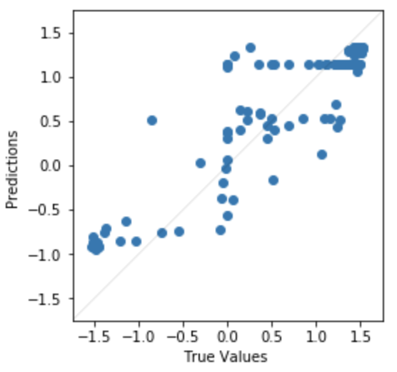
Here it’s evident the model performs better at the minimum and maximum steering command angles than the 0 angle commands.
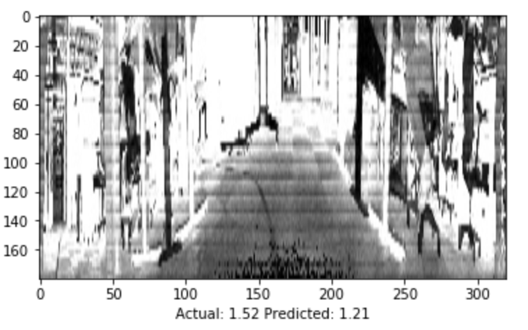
It’s also possible to look at individual images to get a sense of the model’s performance. The image below shows both the precited and true steering angle for a single image.
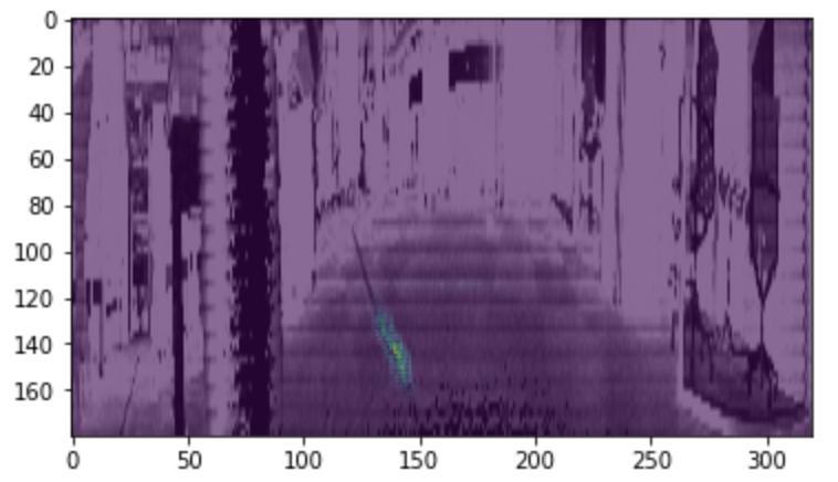
Finally, the visualize_saliency function can be used to generate a heatmap indicating the regions of the image that most contribute towards the model output.
Saliency maps were introduced in the paper “Deep Inside Convolutional Networks: Visualising Image Classification Models and Saliency Maps.” They are based on gradients and they calculate the gradient of the output with respect to each pixel in the input image. This shows how the output changes with respect to small changes in the input image pixels.
grads = visualize_saliency(model,layer_idx,filter_indices=None,seed_input=sample_image_mod,grad_modifier='absolute',backprop_modifier='guided')
In the example image below, it’s evident that the network is most sensitive to pixels near the lane marking.
Model Deployment and Verification
Once the model was trained, it was placed on the embedded device and integrated into the RC car control system. The model predicted steering commands in real-time based on input images from the webcam.
A ROS node was developed that subscribes to the image topics published by the camera and published the control commands that are output from the ML model. The drive_model.py file is used to do this.
The model_control_node is created which subscribes to the /img_node/intensity_image topic for lidar images and publishes control commands on the /platform_control/cmd_vel topic.
For each image received, it is first resized to a 180×320 image. This is the input image size that the model expects for inputs.
self.resized_image = cv2.resize(self.latestImage, (320,180))
For this project, only the steering angle command is estimated. Therefore, the throttle is set at a constant value.
self.cmdvel.linear.x = 0.13
Next, the model processes the input image and returns a predicted steering angle.
self.angle = float(model.predict(image_array[None, :, :, :], batch_size=1))
The predicted output is then limited to the maximum steering inputs allowed by the vehicle.
self.angle = -1.57 if self.angle < -1.57 else 1.57 if self.angle > 1.57 else self.angle
Finally, the steering angle command and the desired throttle values are published as a geometry_msgs/Twist message.
self.cmdVel_publish(self.cmdvel)
The system completes this prediction loop continuously to provide updated steering angle commands to the vehicle.
To launch the complete system, the rc_mlmodel_cam.launch is used. This launch file loads the drive_model.py ROS node in addition to loading the common RC vehicle input and control nodes defined in rc_dbw_cam.launch.
When the system is running, the vehicle can be controlled by two different inputs. The control commands from the Xbox controller are still subscribed to on the /joy_teleop/cmd_vel topic. Additionally, the ML model is publishing control commands on the /platform_control/cmd_vel topic.
The yocs_cmd_vel_mux node serves as a multiplexer for command velocity inputs. It arbitrates incoming cmd_vel messages from several topics, allowing one topic at a time to command the robot, based on priorities. All topics, together with their priority and timeout are configured through a YAML file, that can be reloaded at runtime. This is defined in the rover_cmd_vel_mux.yaml configuration file.
Once the system is properly configured, the RC vehicle is placed on the track and the system is executed using the rc_mlmodel_cam.launch launch file.
$ roslaunch behavior_cloning rc_mlmodel_cam.launch os1:=true ekf:=false
The video below depicts a completely autonomous lap using the model defined in this process. The image recorded by the webcam can be seen as well as an overlay of the saliency image depicting the areas in the image that most contribute towards the steering command output.
This post originally appeared on Wil’s blog: https://www.wilselby.com/2020/02/rc-car-ml-model-development-with-ouster-os1-lidar/#more-9702
Related Articles

Setting a new standard in ITS: Ouster BlueCity with Rev8 steals the show at ITS America
Recap from ITS America in Detroit. Ouster BlueCity with Rev8 brings the world's first native color lidar to traffic management, delivering up to 500 feet of multimodal advance detection, with the first deployment streaming from Stamford, CT.

NJDOT
Ouster BlueCity to be deployed at 42 urban highway locations covering mainline and ramps close to the MetLife Stadium The deployments are part of New Jersey Department of Transportation’s (NJDOT) project representing the largest and fastest Intelligent Transportation System (ITS) deployment in the State’s history.NJDOT’s project integrates Ouster BlueCity into the statewide Advanced Traffic Management System (ATMS) for enhanced mobility and safety.

Nashville 100+ Intersection and Roadway Deployment
Ouster BlueCity to be deployed at 100+ additional intersections and roadways throughout NashvilleExpansion follows successful pilot in north Nashville area and multi-intersection deployment on Broadway for corridor-level analytics and traffic management intelligence