

Making HD Maps with lidar sensors.
One of the best uses of lidar technology is for mapping. With lidar, you get a 3D model of everything around you.
Using SLAM to make HD Maps.
All it takes to make a 3D map of the world is to line up lidar scans taken at different places. The process of lining them up, however, is not so easy. This is especially true if the lidar is mounted on a moving platform, such as a car.
In the past, lidar mapping has relied on a laser scanner mounted on an expensive rig including a high-precision GPS inertial navigation system (INS). Using the position and orientation measured by the GPS INS, you can line up the lidar point clouds. Modern GPS INS systems are very good — using techniques such as ground-based stations with real-time kinematic (RTK) correction signals, GPS INS systems can pinpoint your location to within a few centimeters. This is vastly better than cheap GPS units such as cell phones, which may be off by tens of meters. Unfortunately, good GPS INS systems are very expensive. They often cost tens of thousands of dollars!
At Ouster, we don’t use expensive GPS INS systems for mapping. Buying a GPS INS system, which costs many times as much as an Ouster OS1, would nullify the cost advantages of the OS1 to begin with. Instead, we use the lidar data itself to line things up. This is called simultaneous localization and mapping (SLAM). Previously, computers weren’t fast enough to run SLAM reliably with lidar data, but recent developments in SLAM techniques, as well as faster computer hardware, have now made it possible.
The principle of SLAM is: The best explanation of your sensor data is the simplest one. And the simplest explanation of sensor data is when everything lines up [1].
Measuring how lidar data line up.
Aligning the points
Most robotics algorithms can be summed up in two steps. First, define a function called the loss function, or the objective function, which has a large value when things are bad and a small value when things are good. Second, adjust things to minimize said function.
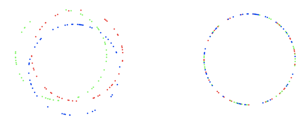
For aligning two point clouds from lidar, we can define the objective function in the following way. Let’s consider moving the measured point cloud M to line up with the static scene point cloud S. For every point in M, we find the closest point in S. Then, the objective function is the sum of squared distances of every point in M to its corresponding point. We try to minimize the objective function by rotating and shifting the point cloud M. The objective function may be minimized using a variety of nonlinear least squares solvers, such as Levenberg–Marquardt [2]. Here, the optimization variables are the rotation and translation of the point cloud M. When working in 3D, rotation and translation have six degrees of freedom in total.
After minimizing the cost function, the point cloud M will have moved, which means that the corresponding closest points may have changed. To deal with that, we simply repeat the procedure until the closest points do not change. This algorithm is called iterative closest point (ICP).
Looking for the closest point works pretty well for mobile mapping vehicles and robots because they move smoothly, so we have a pretty good guess for where they will be. So the closest point initially is quite likely to remain the closest point even after optimization.
In practice, lidars points do not exactly correspond to each other directly. Instead, lidar scans sample points from some underlying physical surface. To take this into account, we may use point-to-plane ICP. Instead of finding one closest point, we find several, and then fit a plane to those points. Then, instead of minimizing distance between a pair of points, we minimize the distance from a point to a plane.
Other advanced methods exist, such as generalized ICP, methods using surfels, or the normal distributions transform, all three of which involve multivariate Gaussian distributions describing the geometry of a local neighborhood of points.
Incorporating other sensors
Every Ouster OS1 has a built-in inertial measurement unit (IMU). This is a low-cost sensor similar to the one found in every smartphone. Though not as accurate as a high precision INS, it is nonetheless incredibly useful.
Just like with aligning points, we can also incorporate IMU data using a similar strategy. First, we formulate an objective function that penalizes the difference between inertial measurements (rotational velocity and translational acceleration). Second, we optimize our state to minimize this objective function.
It turns out that we can combine all of these various objective functions into one big one. This is called a tight coupling. In general, the more sensors, the better!
Real time performance
The Ouster OS1 outputs over 1 million points per second, one of the highest in its class, thanks to its unique multi-beam flash lidar design. Unfortunately, with great resolution comes great computational complexity.
Our SLAM algorithm is notable for being able to run in real time with not just one, but three Ouster OS1 devices at the same time, on a typical desktop computer CPU.
The secret is to not consider all points for the objective function, but only a handful of the best ones. This is known as feature extraction, and the best points are known as feature points.
One way to extract features is to find the points in the flattest part of the point cloud. As mentioned earlier, one objective function strategy is point-to-plane ICP. Intuitively, the points that match well to planes should lay on a plane themselves. We can compute a measure of flatness around every point, by computing the principle component analysis in a small neighbourhood around it. Then, we keep the best, say, thousand flattest points, provided no two of them are too close to each other, to ensure that we get an even distribution of points.
In contrast to geometric feature extraction, it may also be possible to use lidar intensity combined with image-based feature extraction methods. Using the fact that the Ouster OS1 can capture 2D camera-like imagery, we can use deep-learning based feature extraction such as SuperPoint. This makes our algorithm more robust. For example, geometric feature extraction may fail in a smooth tunnel where all the planes point in the same direction, but visual features may still exist due to the texture of tunnel walls.
Continuous time
Conventional SLAM algorithms line up one frame with the next. However, most sensors in the real world do not output discrete frames at a convenient rate. For example, an inertial measurement unit may output data at 1000 Hz, but it wouldn’t be feasible to deal with updating the vehicle’s position 1000 times per second. The Ouster OS1 outputs data at an even higher rate: groups of 64 points arrive at 20,480 times per second. In other words, each 2048×64 frame is spread out over a tenth of a second, where each column of pixels has a slightly different timestamp.
Previous methods for lidar-based SLAM simply apply frame-to-frame point cloud alignment using 0.1 seconds of data. At highway speeds, a car may have moved 3 meters during that time, leading to distortion in the point clouds. Hence, such methods tend to use an external sensor, such as wheel odometry, to “de-warp” the point clouds prior to alignment. Since the wheel odometry is not as accurate as the lidar measurements, the de-warping is never perfect, and will lead to an inaccurate result.
At Ouster, to deal with multiple high frequency sensors which are possibly operating at different rates, we adopt a continuous time approach. Instead of translating and rotating an entire point cloud as though all the points were collected at the same time, we consider the trajectory of the vehicle as a continuous function of time.
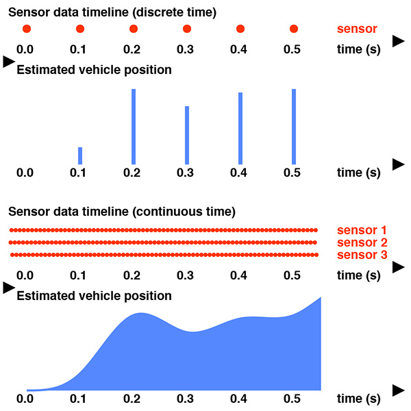
There are two main ways to deal with continuous trajectories. The first one is non-parametric methods such as Gaussian processes (which we won’t get into details here). The second, more popular one is to parameterise the trajectory as a spline function. A popular choice is a cubic B-spline [3], which sees lots of use in the computer graphics industry. With a cubic B-spline, we can store a sequence of spline knots, spaced perhaps 0.1 seconds apart [4]. The value of each knot is 6-dimensional: a combination of rotation and translation. Then, the trajectory at any point in time is the weighted sum [5] of the four closest knots. Using this method, we have a reasonable quantity of optimization variables at only 10 variables per second, rather than thousands. At the same time, motion distortion is no longer a problem.
As for the optimization problem, instead of aligning two frames together, we consider all the points inside a sliding window in time, say, 0.5 seconds [6] long. The window slides forwards 0.1 seconds at a time. Consider all the points in the last half a second — for each of those, we find the several closest points in space, provided they are not too close in time. This gives us the same set of distances, which we can minimize as before. Now, instead of updating the rotation and translation of the whole point cloud, we instead update each of the relevant knots.
As a bonus, since a cubic B-spline is differentiable, it is natural to derive the IMU objective function. This would have been challenging using nondifferentiable representations of the vehicle trajectory.
Closing the loop
So far, we have talked about estimating the trajectory using a sliding window of the most recent 0.5 seconds of data. However, even a highly sophisticated SLAM algorithm using highly accurate sensors will be susceptible to some amount of random uncertainty. As such, the dead-reckoning trajectory found in this way will inevitably drift slightly from the true trajectory of the vehicle. A consequence is that, when driving in a very large loop, the vehicle’s estimated trajectory may not end up in the same spot even when the vehicle has actually returned to exactly where it started out. This is known as the loop closure problem.
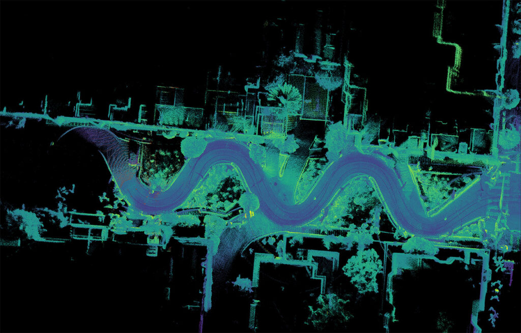
Loop closure is still an active area of research. At Ouster, we’re working on a cutting edge solution to loop closure, using technique based on fast Fourier transforms for place recognition and rough alignment. Then, a large point cloud alignment batch optimization is performed to seamlessly fuse the data from multiple vehicles into one 3D model. The batch optimization is fully containerized, runs on cloud infrastructure and is designed to be highly scalable.
The result is a crisp, detailed 3D map which progressively becomes finer and more accurate as more vehicles drive through the same region.
Conclusion
Large-scale 3D mapping is hard. Ouster is able to make mapping happen at a bigger scale, with better resolution, and for a lower price than anyone else. Ouster’s software-focused mapping strategy obviates the need for high precision GPS systems, wheel odometry, or expensive gyroscopes. Furthermore, the Ouster OS1’s multi-beam flash lidar design is vastly cheaper, smaller, and lighter than any other lidar producing a comparable number of points. This means that Ouster’s mapping system can be deployed easily and cheaply on any platform, be it drones, cars, or robots.
1 A point cloud registration objective function may be shown to be equivalent to entropy, as seen in section 2.2 of Tsin, Y., & Kanade, T. (2004, May). A correlation-based approach to robust point set registration. In European conference on computer vision (pp. 558-569). Springer, Berlin, Heidelberg.
2 https://en.wikipedia.org/wiki/Levenberg%E2%80%93Marquardt_algorithm
3 Piecewise linear functions and Hermite splines are also popular.
4 The spacing of the knots depends on the dynamics of the vehicle. A car’s speed is unlikely to change very much during 0.1 seconds. Also, more knots is more computationally expensive. In general, the time needed scales to the cube of the number of knots.
5 The “sum” in this case requires the mathematical machinery of Lie groups, as rigid transformations in 3D are in the Special Euclidean Group which is non-Euclidean.
6 The longer the optimization window, the more accurate the result. However, a long window is computationally expensive. For robotics applications, it is also important to get low-latency estimates of vehicle position and orientation.
Related Articles

Unlocking Federal Funding for Smart Infrastructure: Ouster BlueCity with Rev8 Achieves BABA Compliance
Ouster BlueCity with Rev8 has achieved system-level BABA (Build America, Buy America) Act compliance, clearing a major procurement hurdle for state and local transportation agencies pursuing federally funded ITS upgrades. The milestone means Ouster's lidar and edge computing hardware meet domestic manufacturing requirements, making BlueCity eligible for deployment in federally funded intersections, corridors, transit networks, and tolling systems. Combined with Rev8's native color lidar, extended range, and 10-year production life, the announcement positions Ouster BlueCity as a low-friction path to modernizing American roadways.

Privacy by Design: How Ouster BlueCity Fuses Native Color Lidar with Edge Privacy
Ouster BlueCity with Rev8 is the industry's first native color lidar detection system, giving traffic engineers up to 500 feet of advance detection and richer situational awareness at intersections. Its edge-processed AI, running on NVIDIA Orin AGX and trained on 4 million labeled objects across 800 sites, delivers 99% stop bar detection accuracy while automatically blurring pedestrians and cyclists to protect identity.

Setting a new standard in ITS: Ouster BlueCity with Rev8 steals the show at ITS America
Recap from ITS America in Detroit. Ouster BlueCity with Rev8 brings the world's first native color lidar to traffic management, delivering up to 500 feet of multimodal advance detection, with the first deployment streaming from Stamford, CT.