Object Detection and Tracking using Deep Learning and Ouster Python SDK

As more companies invest in the field of automation, the need for computers to identify objects and understand their positions in 3D space is growing more important. While the tasks seem pretty simple to humans, the devil lies in the details.

Today, most algorithms to identify objects are achieved with 2D camera images but they lack 3D spatial awareness. While 3D lidar sensors could provide highly accurate 3D information, they don’t have a rich algorithm ecosystem to identify and classify objects. So, can we marry 2D algorithms with 3D spatial awareness?

In this post, we will walk through how to bridge the gap with Ouster lidar sensors. We will demonstrate how to leverage a powerful 2D perception algorithm with 3D spatial data by building a social distancing application. Let’s begin!

Project Overview

Our goal is to identify persons with an OS0-128 lidar sensor and trigger an alarm when the relative distance between the two people is less than 1.8 meters. 

Here’s a preview of the final results. You can see in this short demo video, that the model detects and tracks the people in the scene and calculates the relative distance between the two in real-time. When two people get closer than 1.8 meters, the alarm is triggered and the bounding boxes turn red. 

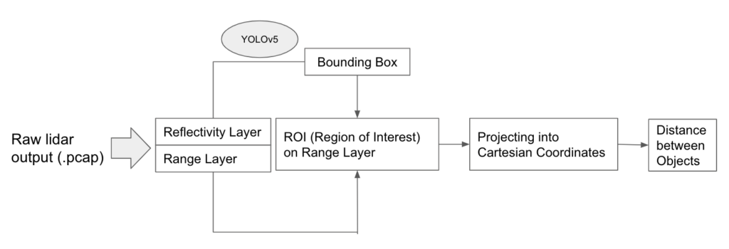
Below is an overview of the pipeline of how we convert the raw point cloud data (.PCAP file) to the distance between the objects. In this post, we will go through the pipeline in detail. 

We highly encourage you to follow along to replicate the results and the following is all you need to do so:

• Our custom YOLOv5 repository for this project (based on the original YOLOv5 repo)
• Ouster Python SDK 
• Sample Data (please download both PCAP and JSON files)

Ouster Data Recap

Before we begin, let’s take a quick look at the unique features of Ouster lidar sensor data that makes this project possible. Understanding Ouster’s rich data layers and its perfect 1:1 spatial correspondence of points is the key to understanding how we are able to combine 2D algorithms and 3D spatial data.

Ouster Data Layer

Our lidar sensor outputs four data layers for each pixel: Range, Signal, Near-IR, and Reflectivity. 

⇒ Range: The distance of the point from the sensor origin, calculated by using the time of flight of the laser pulse

⇒ Signal: The strength of the light returned to the sensor for a given point. Signal for Ouster digital lidar sensors is expressed in the number of photons of light detected

⇒ Near-IR: The strength of sunlight collected for a given point, also expressed in the quantity of photons detected that was not produced by the sensor’s laser pulse

⇒ Reflectivity: The reflectivity of the surface (or object) that was detected by the sensor

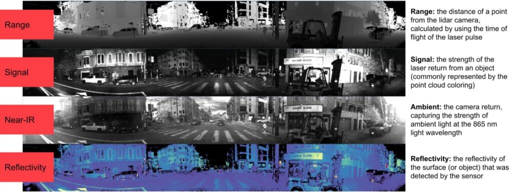
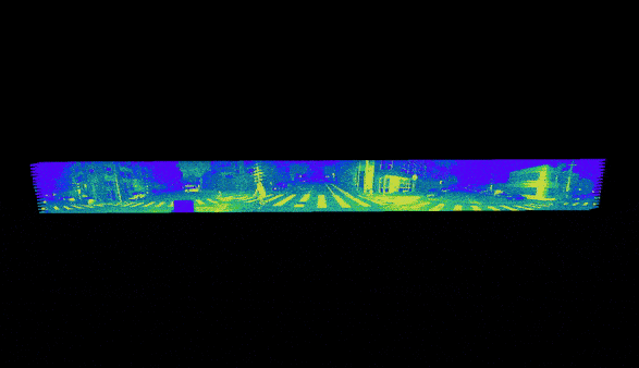
For this project, we utilized the reflectivity layer to identify objects and the range layer to calculate the relative distance between objects. We chose the reflectivity layer for object detection because it contains information about the inherent reflective property of objects. Where signal varies with range (objects further away return less light) and near-IR data varies with sunlight levels (not visible at night or indoors), reflectivity data is consistent across lighting conditions and range. 

Perfect 1:1 Spatial Correspondence of Points 

One of the unique features of Ouster lidars is the 1:1 spatial correspondence of points. Each pixel in a structured 2D image represents a 3D point in our sensor natively without any discretization or resampling. As a result, no unnecessary noise or artifacts are added to the perception pipeline which helps boost accuracy while reducing the computational needs significantly. This is a huge advantage when combining the strengths of 2D images and 3D spatial recognition.

Because the sensor outputs fixed resolution image frames with range, signal, reflectivity, and near-IR data at each pixel, we’re able to feed these images directly into deep learning algorithms that were originally developed for cameras. 

Now that we are more familiar with Ouster’s unique lidar data, let’s get started!

YOLOv5 + Ouster

For our social distance project, we decided to work with YOLOv5, which is a lightweight Convolutional Neural Network (CNN) based object detection algorithm. YOLOv5 is one of the popular 2D perception algorithms due to its fast speed (up to 100+ frames per second inference speed with GPU) and high accuracy. However, it does not work with the Ouster data format (PCAP file). Hence, the starting step would be to modify YOLOv5 so that it can read our reflectivity layer and detect objects, specifically humans. 

Object Detection with YOLOv5 

Before we dive deeper, let’s learn how to use YOLOv5 to detect an object from an RGB image. 

First, let’s clone the repository and install the required packages in a Python>=3.7.0 environment, including PyTorch>=1.7.

git clone https://github.com/fisher-jianyu-shi/yolov5_Ouster-lidar-example 
cd yolov5_Ouster-lidar-example #go to source directory
pip install -r requirements.txt  #install required packages

The detect.py file (from the original YOLOv5 repo) in the source directory runs inference on a variety of sources (images, videos, video streams, webcam, etc.). For example, to detect people in an image using the pre-trained YOLOv5s model with a 40% confidence threshold, we simply have to run the following command in a terminal in the source directory:

python detect.py --class 0 --weights Yolov5s.pt --conf-thres=0.4 --source example_pic.jpeg --view-img 

--class 0: #detection class (0 = people)
--weights Yolov5s.pt #pre-trained weights; s stands for small. 
You can also try the smaller model YOLOv5n, or bigger models like YOLOv5m/l/x  
--conf-thres=0.4 #confidence threshold, any prediction with a confidence level lower than specified 
will not be considered a valid prediction
--source example_pic.jpeg #path to the image; can also be video, stream, webcam--view-img #show results

This will automatically save the results in the directory runs/detect/exp as an annotated image with a label and the confidence levels of the prediction. 

YOLOv5 + Ouster using Ouster Python SDK

As mentioned earlier, YOLOv5 takes an image, video, webcam, or video stream, but it does not recognize PCAP files generated by Ouster lidar sensors. To feed Ouster data to YOLOv5, we need to transfer its data layers into images. Luckily, the Ouster Python SDK makes this task extremely easy. With the help of the SDK, we modified the detect.py file to run the inference on the reflectivity layer from the PCAP file. The modified detection script is called detect_pcap.py. 

Let’s install the Ouster Python SDK (follow the installation instructions here), download the sample data, save both the PCAP and JSON files in the source directory, and run the following command: 

python detect_pcap.py --class 0 --weights yolov5s.pt --conf-thres=0.4 
--source Ouster-YOLOv5-sample.pcap --metadata-path Ouster-YOLOv5-sample.json --view-img

You should see a video automatically generated in runs/detect/exp.

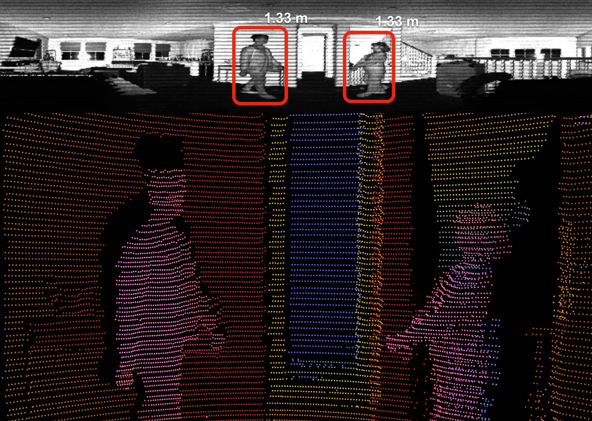
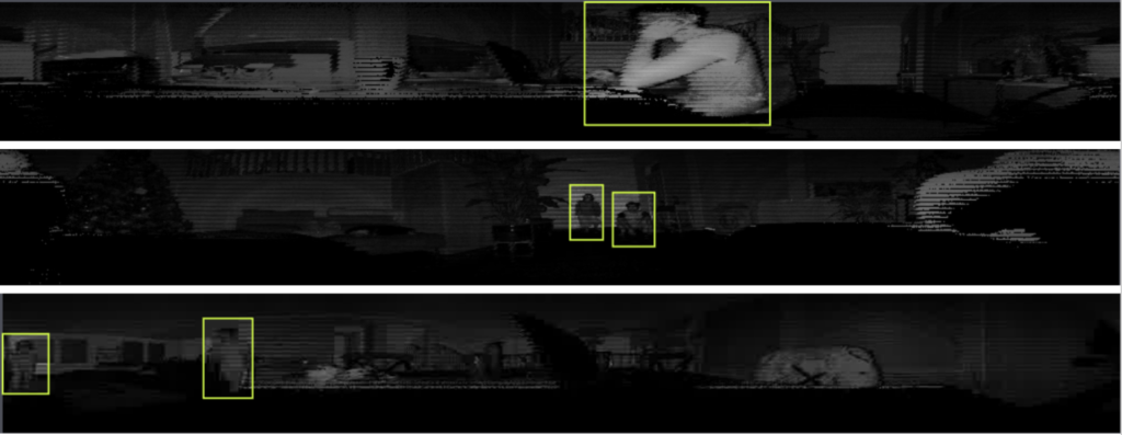
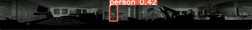
Even though YOLOv5 was never trained with lidar reflectivity data, the model shows promising performance. It shows that we can directly apply algorithms trained on camera images to the reflectivity data lidars. There’s a lot of room for improvement of course. As we can see in the screenshot below, with the default YOLOv5s weights, a person was identified with a confidence level of 42% (barely over the 40% threshold), but the other person is missing. 

Let’s go through how we did this in more detail. 

Our lidar sensor provides two files: a PCAP file which is raw UDP packets captured by the sensor, and a JSON file which contains the sensor’s metadata that’s required to interpret packets. Using the SDK, we first loaded the sensor metadata using the client module.

from ouster import client 
metadata_path = '<DATA_JSON_PATH>'
with open(metadata_path, 'r') as f:
    metadata = client.SensorInfo(f.read())

With the metadata, we can now read the PCAP file by instantiating pcap.Pcap using the pcap module:

from ouster import pcap
pcap_path = '<DATA_PCAP_PATH>'
pcap_file = pcap.Pcap(pcap_path, metadata)

Now, let’s parse the PCAP into individual scans using the Scans module. A scan is a restructured 360º view of data. Since we’ll be using the reflectivity and range layers, let’s pull them out from each scan. The calls look like the following:

import numpy as np

with closing(client.Scans(PCAP_file)) as scans:    
    for scan in scans:
    ref_field     =scan.field(client.ChanField.REFLECTIVITY)  
    ref_val = client.destagger(PCAP_file.metadata, ref_field) #the destagger function is to adjust for the pixel 
staggering that is inherent to Ouster lidar sensor raw data         
    ref_img = ref_val.astype(np.uint8) #convert to numpy array for image processing later 

    range_field = scan.field(client.ChanField.RANGE)      
    range_val = client.destagger(PCAP_file.metadata, range_field)

One thing to point out is the destagger function. Many of you might already know, but a rotating lidar doesn’t capture the whole picture at once. Since beams are fired and received at different angles at different moments, a raw image captured by a lidar is fuzzy or staggered. However, the metadata file contains when and where the packets were received, allowing us to reconstruct and destagger the raw data into an accurate visual representation. For more details about staggered vs destaggered scans, check out this page. 

Retrain YOLOv5 with Lidar Data

The default model was trained on the COCO dataset, which contains mostly RGB images. Moreover, the shape of the reflectivity image (e.g. 512/1024/2048 x 128) is quite different from that of a typical image (e.g. 640 x 640) the YOLOv5s model was trained on. Therefore, it is not surprising to see that the performance on the reflectivity image is not as good as a typical RGB image.

Let’s see if we can retrain the model with some custom data and improve the performance. To retrain the YOLOv5 model with lidar data, we need to build our own training data set.

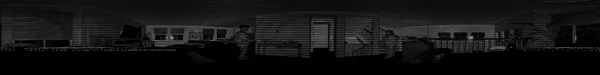
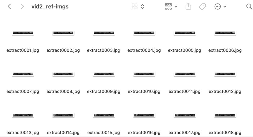
Get Training Images from PCAP Files

We collected multiple PCAP files with an OS0-128 (you can see how to do it here), and then used the Ouster Python SDK to pull the reflectivity layer of each scan and utilized OpenCV’s cv2.imwrite function to save the reflectivity layers as grayscale images for data labeling:

import cv2
import numpy as np
from contextlib import closing
from ouster import client
from ouster import pcap

with open(metadata_path, 'r') as f:  
    metadata = client.SensorInfo(f.read())

source = pcap.Pcap(pcap_path, metadata)

counter = 0

with closing(client.Scans(source)) as scans:        for scan in scans:
        counter += 1 
        ref_field = scan.field(client.ChanField.REFLECTIVITY)
        ref_val = client.destagger(source.metadata, ref_field)
        ref_img = ref_val.astype(np.uint8)

        filename = 'extract'+str(counter)+'.jpg'    
        cv2.imwrite(img_path+filename, ref_img)

We could do more, but for the sake of time, we generated a small data set of 700+ reflectivity images.

Data Labeling

Now it’s time to label the reflectivity images for training. YOLOv5 integrates with Roboflow, which is a free-to-use tool to organize, label, and host datasets. Data labeling could be a tedious job, but Roboflow made our life much easier with its web-based GUI and seamless integration with YOLOv5.  

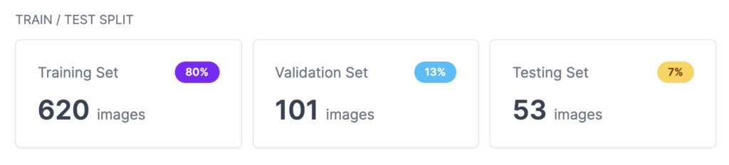
After the labeling was done, the dataset was split into a training, validation, and testing set with 80% in the training set. 

Training using Google Colab

Now that we have the dataset, let’s start the training! We used the YOLOv5_train_Ouster.ipynb Jupyter notebook to train our custom weights. This notebook is a slightly modified version of the official YOLOv5-Custom-Training notebook.  

The training was done using a GPU-enabled Google Colab account. To train the model on the custom-labeled data, we used the Roboflow Python package to download the data to the Google Colab workspace:

from roboflow import Roboflow
rf = Roboflow(model_format="yolov5", notebook="ultralytics")

This will generate a link to get an API KEY. After getting the API KEY, the following code will start the downloading of the labeled dataset hosted by Roboflow: 

rf = Roboflow(api_key="YOUR API KEY HERE")
project = rf.workspace().project("YOUR PROJECT")
dataset = project.version("YOUR VERSION").download("yolov5")

Now with the dataset downloaded, we can use the train.py file (from the original YOLOv5 repo) to train the model with our own data. We used transfer learning based on pre-trained YOLOv5s weights so that we don’t need to train the weights from scratch. 

We trained the weights with a batch size of 16 for 30 epochs:

​​!python train.py --img 640 --single-cls --batch 16 --epochs 30 --data '<DATA_PATH>' --weights yolov5s.pt --cache

With a GPU instance (Tesla P100-PCIE-16GB), the training took just about 7 minutes!.  

Inference using Custom Trained Weights

After the training is done, the newly retrained weights with the best performance are automatically stored as best.pt in runs/train/exp/weights/. Let’s try the new weights and see if it performs better than the pre-trained YOLOv5s weights:

python detect_pcap.py --class 0 --weights best.pt --conf-thres=0.4 --source Ouster-YOLOv5-sample.pcap --
metadata-path Ouster-YOLOv5-sample.json  --view-img

Let’s see how it looks with the custom-trained model:

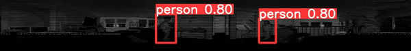
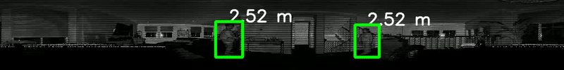
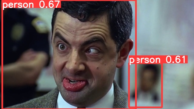
There’s a pretty significant improvement with custom training! Below is a comparison of the perception performance between pre-trained (top image) and custom-trained YOLOv5s (bottom image). 

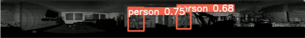
As we can see in the screenshot above, the custom-trained model now identifies two people, not one, with higher confidence levels in both. 

If we wanted to further optimize the object detection performance, two obvious routes would be to train with more training data and train with a bigger network (YOLOv5m or YOLOv5l for example. One thing to keep in mind is that the bigger the network, the longer it takes to do training and inference). For the sake of this example, let’s say this is good enough and move on to calculating the distance between the two people.

Relative Distance Calculation

Now let’s calculate the distance between the people detected.  

Here’s a picture illustrating how we did the relative distance calculation: 

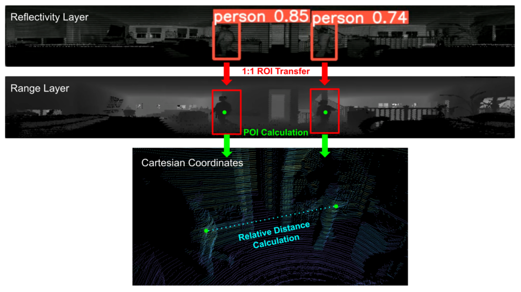
Let’s go through the details. 

Because of the perfect 1:1 spatial correspondence of points, each pixel in the 2D image can be easily translated into Cartesian Coordinates using the Ouster Python SDK and the metadata. There is a precomputed lookup table that is included in the metadata file to project each pixel into Cartesian Coordinates:

from ouster import client

xyzlut = client.XYZLut(metadata) #call cartesian lookup table
xyz_destaggered = client.destagger(metadata, xyzlut(scan)) #to adjust for the pixel staggering that is 
inherent to Ouster lidar sensor raw data

Now that we have the X, Y, Z coordinates of each point in the scan, let’s find the range values inside the bounding boxes, or regions of interest, created above. All we need to do is to take the (x,y) coordinates of the bounding boxes in the reflectivity layer, and use the same (x,y) coordinates in the range layer to get the range readings that we care about. 

range_roi = range_val[int(xyxy[1]):int(xyxy[3]), int(xyxy[0]):int(xyxy[2])] #xyxy is the X Y coordinates of 
the bounding box

Inside the range_roi matrix, we have all the range values inside the bounding box. To make things simple, we’ll be taking a shortcut by picking the point of interest (POI) that is the closest point to the sensor within each bounding box to represent the identified person. 

poi = np.unravel_index(range_roi.argmin(), range_roi.shape) #take the (x,y) coordinates of closest point within roi 

For each bounding box, we now have a point to represent the person detected. We can easily find the X, Y, Z coordinates of the point using the precomputed lookup table:

xyz_val = xyz_destaggered[poi] #get the (x,y,z) coordinates with the lookup table
xyz_list.append(xyz_val) #save the (x,y,z) coordinates for distance calculation

With the X, Y, Z coordinates of these points saved in xyz_list, let’s calculate the distance between two identified people. 

xyz_1 = xyz_list[0] #person 1 coordinates (closest point in bounding box 1)
xyz_2 = xyz_list[1] #person 2 coordinates (closest point in bounding box 2)
dist = math.sqrt((xyz_1[0] - xyz_2[0])**2 + (xyz_1[1] - xyz_2[1])**2 + (xyz_1[2] - xyz_2[2])**2) #distance 
between two X Y Z coordinates)

With a social-distance argument added in detect_pcap.py for the relative distance calculation, let’s try it out:

python detect_PCAP.py --class 0 --weights best.pt --conf-thres=0.4 --source Ouster-YOLOv5-sample.pcap 
--metadata-path Ouster-YOLOv5-sample.json  --view-img --social-distance

Here’s the final result: 

Closing Thoughts

The social-distancing project demonstrates how you can use an Ouster lidar as a camera and use its accurate depth information for each pixel directly through the Ouster Python SDK. This is just a quick and simple example of how computer vision algorithms can be directly combined with lidar data. Since this project is just a proof of concept, we’ve made some shortcuts in the interest of time. There are some areas that we can improve upon:

• The custom weights of the YOLOv5s model were trained with only 700 images. We could try collecting more data to increase the accuracy in different scenes. 
• We could try adjusting the colorspace and aspect ratio of the reflectivity layer to further improve the detection accuracy.
• We used the pixel within the bounding box that is closest to the sensor. Obviously, this would not work if there is an object between the detected person. To make the distance calculation more robust, we could try subtracting background points within each bounding box and calculate the center of mass of each person.
• Currently, the code only works with recorded data. We could try adding the capability to do object detection and distance calculation from an Ouster lidar live stream.

However, this is still a very good demonstration of how Ouster Python SDK empowers lidar users to utilize 2D machine learning algorithms with rich 3D spatial information. Imagine what else you could do. Some ideas we had are:

• You could try training the YOLOv5 model with 3 layers (e.g. reflectivity + range + near-IR) instead of a single layer to potentially improve the perception performance.
• You could try using YOLOv5 to detect other objects (e.g. vehicle, cyclist, and pedestrian) and calculate their distance and speed for accident detection at intersections.
• You could play with bigger YOLOv5 models (e.g. YOLOv5x) for better accuracy or smaller YOLOv5 mode (e.g. YOLOv5n) for better inference speed. 
• You could try other 2D object detection models (e.g. Object Detection with Transformers) or 2D pixel-wise Semantic Segmentation models (e.g. Nvidia LidarNet). 

If you want to give it a try more and contribute, head on over to our GitHub page. We’d love to see what you can create!